Multiplying (73) by an arbitrary weight function v(x) and
integrating over the interval [a,b] one obtains
![]()
Evidently (73) and (75) are equivalent, because v(x) is an arbitrary
function. Now we seek a numerical solution to (75), (74) in the form
![]()
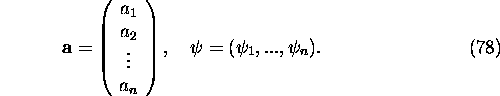
Here ![]() , ...,
, ..., ![]() are functions of x and a1,
..., an are unknown coefficients.
are functions of x and a1,
..., an are unknown coefficients.
In vector form (76) becomes
![]()
where
In (75) we may substitute u by u* to obtain
![]()
However, substituting u(x) by its approximation u*(x) in
(73), generally it appears that (73) is not satisfied exactly, e.g.
![]()
Here e(x) is a measure for the error.
It follows from (79)-(80) that
![]()
Obviously, the residual, e(x), depends on the unknown parameters
given by vector ![]() . Therefore the coefficients a1, ..., an
must be determined so, that expression (81) is satisfied.
. Therefore the coefficients a1, ..., an
must be determined so, that expression (81) is satisfied.
Generally
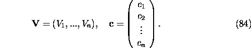
![]()
where V1, ..., Vn are known functions of x and c1, ..,
cn are certain parameters. In terms of vector notation
(82) reads
![]()
where
Evidently
![]()
and therefore (see (81))
![]()
Relation (86) holds for arbitrary cT- matrices, i.e.
![]()
or
![]()
Now, we have n equations (88) to determine coefficients
a1,...,an. Inserting (77) in (80) yields
![]()
and the condition (86) can be rewritten as
![]()
Introducing the matrix K and the vector ![]() as
as
![]()
we can write (90) in compact form
![]()
Finally, we have n linear equations (92) for determing n
coefficients a1,...,an.