An updated, revised, and more readable version of this page can be
found in the math section of this
website.
Spectral Analysis of Mandelbrot Interior
The term 'spectral' or 'characteristic' analysis refers to a way of
understanding the behavior of an infinite sequence by examining the
behavior of various series built up from the sequence.
It is occasionally used to examine the eigenvalues of infinite-dimensional
representations.
In particular, this technology is useful when dealing with divergent
or non-convergent series. The basic idea consists of examining
the analytic properties of a different, 'regulated', series.
Consider the sequence {a0, a1, a2,...}
Then, for small and positive t, construct the sum
S(t) = Sumn=0inf an exp (-tn)
We call this sum the 'regulated' series.
For large class of reasonably behaved series {an}
this sum is finite for all positive values of t.
(By 'reasonably behaved' we mean a sequence where an doesn't
get exponentially large with increasing n; that is, one where the sum
converges.).
The spectral analysis consists of exploring the behavior of the sum
in the limit of t->0. Depending on the series, it may diverge. For
example, if we take all an to be one, the sum
N(t) = Sumn=0inf exp (-tn)
diverges as 1/t, while
Sumn=0inf n exp (-tn)
diverges as 1/t2. We can understand the series better by
understanding the type of divergences it has.
Another common regulator is the (Reimann) zeta regulator:
C(s) = Sumn=0inf an / sn
which is explored in the limit of s->1. Note that S(t) can be derived
from C(s), and v.v., through analytic means. In particular, poles in
the complex s-plane map to powers of t; if C(1) is finite, then so is
S(0) and v.v. However, S(t) is far easier to deal with computationally
than C(s) is. In fact, to further simplify the numerical calculations,
we'll use the regulator exp (-t2n2), which
converges a good bit faster. It also can be analytically related to
the other regulators.
This page is devoted to the application of these sums to the Mandelbrot
series: zn+1 = zn2+c. Let us then
consider
S(t) = Sumn=0inf zn exp (-t2n2)
For most of the interior of the Mandelbrot set, this sum diverges as
1/t. To render an image of this, let
N(t) = Sumn=0inf exp (-t2n2)
which also diverges as 1/t. We use this to show the divergence:
the image below shows limt->0 |S(t)|/N(t)
where |S(t)| is just the modulus of S(t); that is,
|S(t)| = sqrt ((Re S(t))2 + (Im S(t))2)
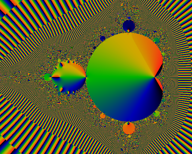
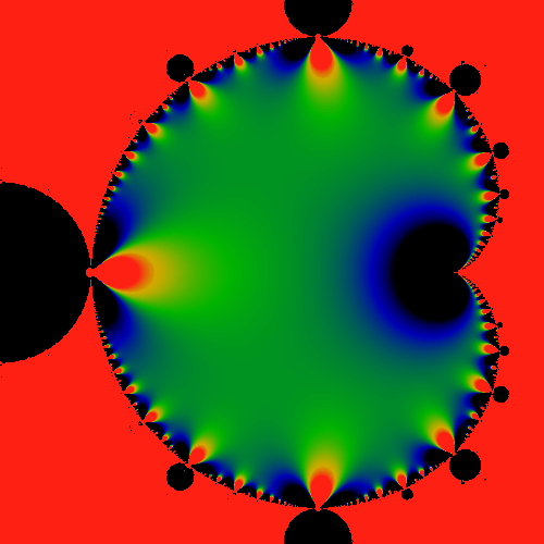
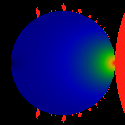
 The color green represents a value of 0.5. Thus, it seems that the
limit has a simple zero at Re c = Im c = 0. The sum is exactly
equal to 1/2 in the largest bud on the left, and approximately
equal to 1/2 in the other buds. Below, we will provide an exact
expression for the divergent term throughout the interior.
The color green represents a value of 0.5. Thus, it seems that the
limit has a simple zero at Re c = Im c = 0. The sum is exactly
equal to 1/2 in the largest bud on the left, and approximately
equal to 1/2 in the other buds. Below, we will provide an exact
expression for the divergent term throughout the interior.
Its somewhat more interesting to look at a related sum, the sum over
second derivatives of z w.r.t. c.
If we write the iterated Mandelbrot equation as so:
zn+1 = zn2 + c, then, realizing that it
is parameterized by c, we can take its derivative:
z'n+1 = dzn+1/dc = 2 z'n zn + 1.
The second derivative follows:
z''n+1 = d2zn+1/dc2 =
2 (z''n zn + z'n2).
Note that zn, z'n and z''n are well
defined for all values of c and finite n: they are entire functions,
'merely' polynomials in c.
We then define the sum:
P(t) = Sumn=0inf z''n
exp (-t2n2).
Note that
P(t) = d2 S(t) / dc2 holds for all positive t.
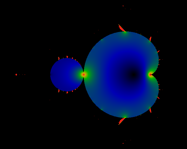
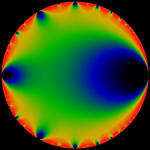
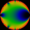
P(t) also diverges as 1/t. The image below shows
limt->0 |P(t)| / N(t)
 Red denotes any value equal or greater than 1.
We can give an exact expression for
limt->0 |P(t)| / N(t)
in the main body. It is
limt->0 |P(t)| / N(t) = 1/( 4 |1/4 - c|3/2 )
(It is numerically straightforward to verify that this expression is
exact to between 6 and 10 decimal places. See the section 'numerical
hints' below for a greater discussion).
The value of this limit in the largest bud to the left is precisely
zero over the entire bud. For the next smallest buds (at the top,
bottom, and the second to the left), the value seems to be uniformly
1/30 across the whole bud, although there does seem to be a slight
gradation which is hard to distinguish from numerical errors. By looking
at this image, we can see that this limit seems to take on other,
constant, values in the progressively smaller buds. The color scheme
here has black <= 0.0, blue ~= 0.2, green ~= 0.5, yellow ~= 0.75,
red >= 1.0. If the values were indeed constant over the smaller buds,
this would have some interesting implications on the limit-cycles
for these buds, as discussed below.
Red denotes any value equal or greater than 1.
We can give an exact expression for
limt->0 |P(t)| / N(t)
in the main body. It is
limt->0 |P(t)| / N(t) = 1/( 4 |1/4 - c|3/2 )
(It is numerically straightforward to verify that this expression is
exact to between 6 and 10 decimal places. See the section 'numerical
hints' below for a greater discussion).
The value of this limit in the largest bud to the left is precisely
zero over the entire bud. For the next smallest buds (at the top,
bottom, and the second to the left), the value seems to be uniformly
1/30 across the whole bud, although there does seem to be a slight
gradation which is hard to distinguish from numerical errors. By looking
at this image, we can see that this limit seems to take on other,
constant, values in the progressively smaller buds. The color scheme
here has black <= 0.0, blue ~= 0.2, green ~= 0.5, yellow ~= 0.75,
red >= 1.0. If the values were indeed constant over the smaller buds,
this would have some interesting implications on the limit-cycles
for these buds, as discussed below.
The next image shows the phase of P(t) in the limit of t->0.
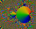 That is, it shows
limt->0 arctan (Im P(t) / Re P(t)).
The color scheme is such that black=-pi, green=0, red=+pi.
Combining what we've learned from this and the previous image,
we conclude that the divergent part of P(t) is precisely
1/( 4 (1/4 - c)3/2 )
That is, it shows
limt->0 arctan (Im P(t) / Re P(t)).
The color scheme is such that black=-pi, green=0, red=+pi.
Combining what we've learned from this and the previous image,
we conclude that the divergent part of P(t) is precisely
1/( 4 (1/4 - c)3/2 )
Since P(t) = d2 S(t) / dc2, we can integrate to
find the divergent part of S(t).
We find that
limt->0 |S(t)|/N(t) =
A(c) = 1/2 - (1/4 - c) 1/2.
Note that |A(c)|=1/2 on the cardiod: we can easily verify that
|A (eip/2 - e2ip/4) | = 1/2 for all values of p.
Next, we note that A(c) is a solution to the Mandelbrot equation:
A(c) = A(c)2 + c. Indeed, this should not be a surprise:
The divergent term of the sum S(t) is in effect the average over
over all values of zn. Inside the main bulb, we have
lim n->inf zn = A(c), and so of necessity,
the leading divergence of the sum must be A(c). Similarly, in
the large bud on the left, zn converges to a two-cycle,
with
zn -> -1/2 + i sqrt (c + 3/4)
and
zn+1 -> -1/2 - i sqrt (c + 3/4) .
The average of these two values is -1/2, and so we can trivially deduce
that
limt->0 S(t)/N(t) = -1/2
and that
limt->0 |S(t)|/N(t) = 1/2
which exactly matches our numerical results.
In other buds, the sequence converges to m-cycles. Thus, in other buds,
the divergent term will be the average over these m values of the limit
cycle. Provided one can calculate this average, then one has an
exact expression for the divergences of S(t).
Let us now turn to the finite remainders.
By subtracting away the divergent pieces, we are essentially subtracting
away the contribution of the asymptotic limit cycle. The remaining
finite parts indicate how the asymptotic behaviour is approched. If the
finite part is large, this indicates that the iteration took a long time
to approach the asymptotic limit. If the finite part is small, then
the series converged to its limit cycle quickly.
 This image shows
limt->0 |S(t)|- A(c) N(t) .
(We take A(c) to be 1/2 in the largest bud).
The color ramp has been scaled by -1: i.e. black = 0, green ~= -0.5,
red <= -1.0. There appear to be a number of poles arrayed along the
perimeter.
This image shows
limt->0 |S(t)|- A(c) N(t) .
(We take A(c) to be 1/2 in the largest bud).
The color ramp has been scaled by -1: i.e. black = 0, green ~= -0.5,
red <= -1.0. There appear to be a number of poles arrayed along the
perimeter.
Lets take an up-close look at the large bud.
 The sum P(t) doesn't have a divergent piece in the large bud.
This image shows
limt->0 |P(t)|
for the area Re c = [-1.25, -0.75].
As can be seen, it has a much more complicated structure. There seem
to be poles located where-ever some horns come together, and sequences
of zeros inside the bud. The poles all seem to have positive residues.
The color ramp has been scaled by ten: i.e. black = 0, green ~= 5,
red >= 10.
The sum P(t) doesn't have a divergent piece in the large bud.
This image shows
limt->0 |P(t)|
for the area Re c = [-1.25, -0.75].
As can be seen, it has a much more complicated structure. There seem
to be poles located where-ever some horns come together, and sequences
of zeros inside the bud. The poles all seem to have positive residues.
The color ramp has been scaled by ten: i.e. black = 0, green ~= 5,
red >= 10.
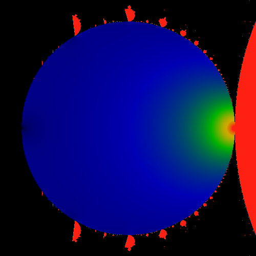
Below is the finite part of S(t) in the largest bud.
 The image below shows
limt->0 |S(t)| - 0.5*N(t)
for the area Re c = [-1.3, -0.7].
It seems to have a simple structure, with a pole at c=(-0.75,0) and a
zero at c=(-1.25,0). Looking more closely, one seems to see zero's
arrayed along the perimeter. In fact, we can expect a rather complex
structure: after all, P(t) = d2 S(t) / dc2 is an
exact identity for any positive t, and we saw that the structure of
P(t) is quite complex.
The color ramp has been scaled by -1: i.e. black = 0, green ~= -0.5,
red <= -1.0.
The image below shows
limt->0 |S(t)| - 0.5*N(t)
for the area Re c = [-1.3, -0.7].
It seems to have a simple structure, with a pole at c=(-0.75,0) and a
zero at c=(-1.25,0). Looking more closely, one seems to see zero's
arrayed along the perimeter. In fact, we can expect a rather complex
structure: after all, P(t) = d2 S(t) / dc2 is an
exact identity for any positive t, and we saw that the structure of
P(t) is quite complex.
The color ramp has been scaled by -1: i.e. black = 0, green ~= -0.5,
red <= -1.0.
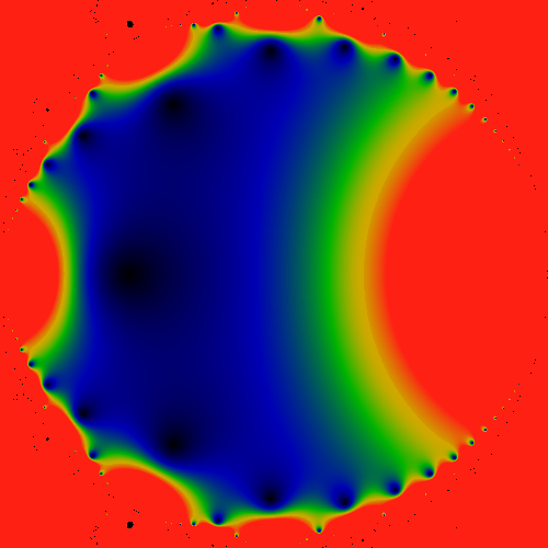
The image below shows the finite piece in the main bulb, after the
divergent piece has been subtracted.
 That is, it shows
limt->0 |P(t)| - N(t) / ( 4 |1/4 - c|3/2 )
It appears to have dipoles (saddles) arrayed along the
perimeter. There don't seem to be any simple zeros.
The color scheme has been adjusted so that black <= -10, green ~= 0
and red >= 10. These (multi-)poles visually indicate something that
is commonly known: the series has a hard time converging near the
tips of the horns.
That is, it shows
limt->0 |P(t)| - N(t) / ( 4 |1/4 - c|3/2 )
It appears to have dipoles (saddles) arrayed along the
perimeter. There don't seem to be any simple zeros.
The color scheme has been adjusted so that black <= -10, green ~= 0
and red >= 10. These (multi-)poles visually indicate something that
is commonly known: the series has a hard time converging near the
tips of the horns.
Visually, this term appears to be some sort of q-series
(q-pochhammer symbol) or Dedekind eta, which is immediately obvious if
we compare to a figure of the Dedekind eta, below.
 This image shows the Dedekind eta. The visual similarity is remarkable.
In particular, this helps confirm the modular group symmetry of the
Mandelbrot set in a rather direct way, and gives us a pretty good idea
of what conformal map is needed to
establish an explicit symmetry.
The Dedekind eta shows up in the theory of modular forms, which has
seen a lot of activity due to thier connection to many very interesting
mathematical topics.
Please see the math section of this
website for a detailed exposition of this relationship.
This image shows the Dedekind eta. The visual similarity is remarkable.
In particular, this helps confirm the modular group symmetry of the
Mandelbrot set in a rather direct way, and gives us a pretty good idea
of what conformal map is needed to
establish an explicit symmetry.
The Dedekind eta shows up in the theory of modular forms, which has
seen a lot of activity due to thier connection to many very interesting
mathematical topics.
Please see the math section of this
website for a detailed exposition of this relationship.
Numerical Hints
Note that the series explored on these pages can be slow to converge,
especially near the 'horns' of the Mandelbrot set. We can improve
things numerically a bit with a trick to extrapolate to t=0.
We do this by working with a Taylor expansion of the
regulator about finite t, and performing sums with that. The sums
can then be recombined in the Taylor expansion, evaluated at t=0.
This technique helps hasten convergence. Working to the second
derivative seems sufficient.
Note that it is wise to double-check one's work against the simplest
sums. This is because working with the Taylors series requires one to
keep a half-dozen or more sums, and to properly combine first and
second derivatives of square-roots, products, and ratios. Easy enough
on paper, but still prone to algebraic errors or typing errors when
writing the code.
Once one has working expressions, it is fairly straightforward to
confirm numerical behavior. For example, when we give lim t->0 results
in the text above, one can see numerically that these results really
are quite accurate, from between five and ten decimal places,
typically.
Authored by Linas Vepstas
linas@linas.org
November 2000.
Copyright © 2000 Linas Vepstas

Spectral Analysis of Mandelbrot Interior
by Linas Vepstas is licensed under a
Creative Commons
Attribution-ShareAlike 4.0 International License.
 The color green represents a value of 0.5. Thus, it seems that the
limit has a simple zero at Re c = Im c = 0. The sum is exactly
equal to 1/2 in the largest bud on the left, and approximately
equal to 1/2 in the other buds. Below, we will provide an exact
expression for the divergent term throughout the interior.
The color green represents a value of 0.5. Thus, it seems that the
limit has a simple zero at Re c = Im c = 0. The sum is exactly
equal to 1/2 in the largest bud on the left, and approximately
equal to 1/2 in the other buds. Below, we will provide an exact
expression for the divergent term throughout the interior.