Everyone (well, almost everyone) knows what an arithmetic function is. They are one of the prime objects of study in number theory; some of the famous ones include Euler's totient function, the Möbius function, the Divisor function, and many, many more. These have many interesting and important relationships between one-another when they are placed into a Lambert series or a Dirichlet series. Many of these relations can be understood by studying modular forms, such as the Dedekind eta function, or the Eisenstein series. Due to the modular symmetry of those functions, one can draw many pretty fractal-shaped pictures of these: Indeed, I supplied many of the pictures used in Wikipedia articles for these topics. I have yet more, in the Numberetic Gallery in this art gallery. I also have numerous writings about the modular group SL(2,Z) on this website, exploring it's fractal symmetry.
So, such series are interesting things to study. However, no one every studies the ordinary or exponential generating functions for these series. Why is that? Perhaps for these reasons?
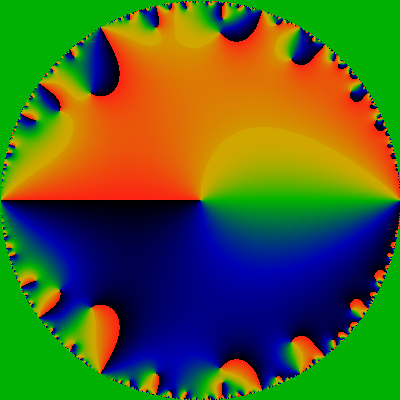
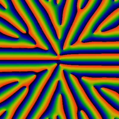
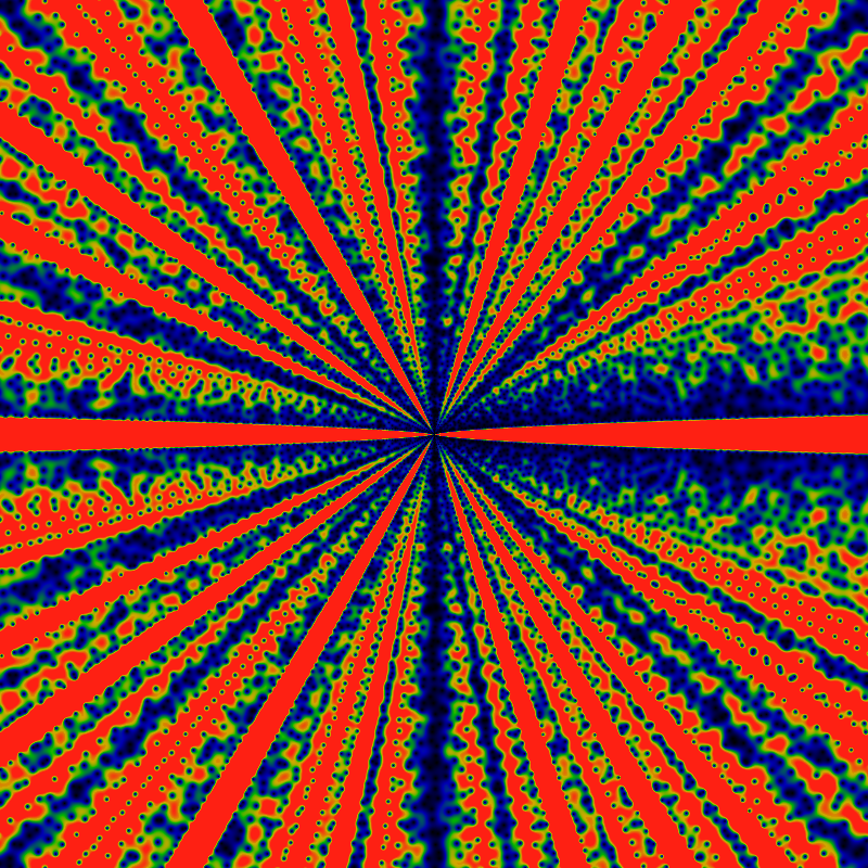
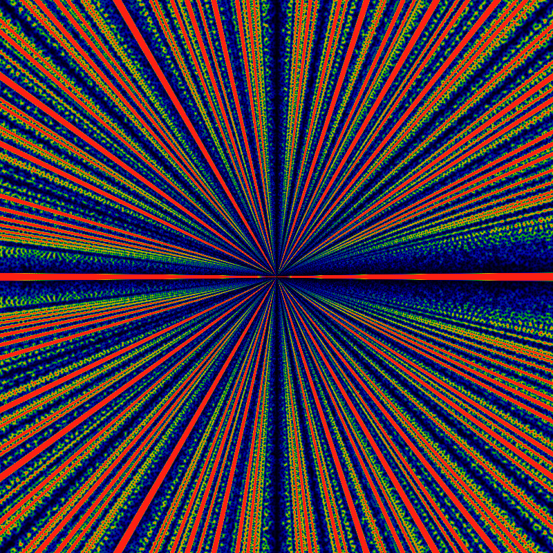
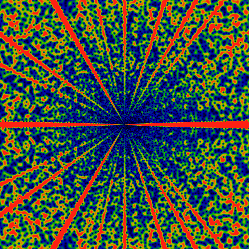
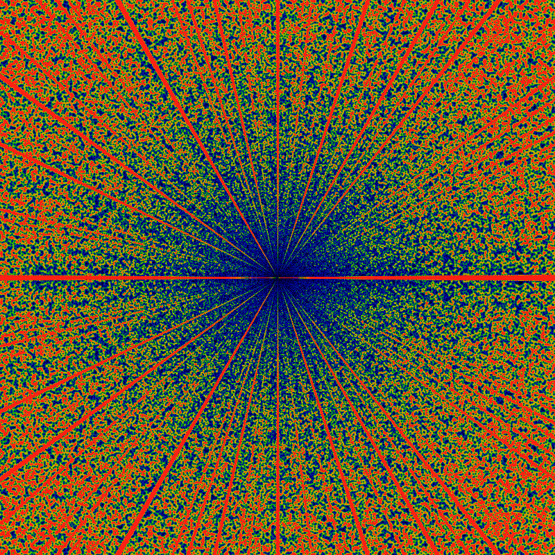
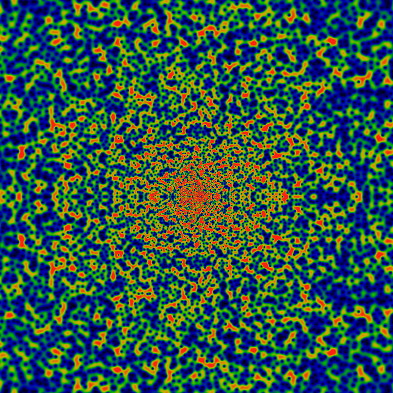
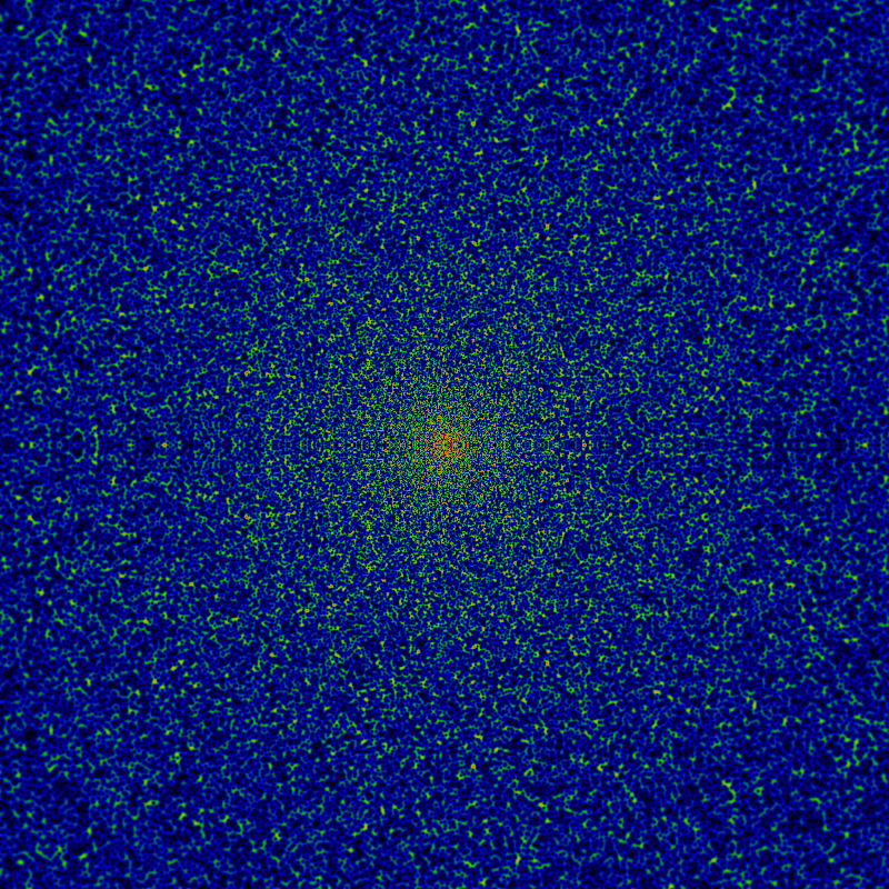
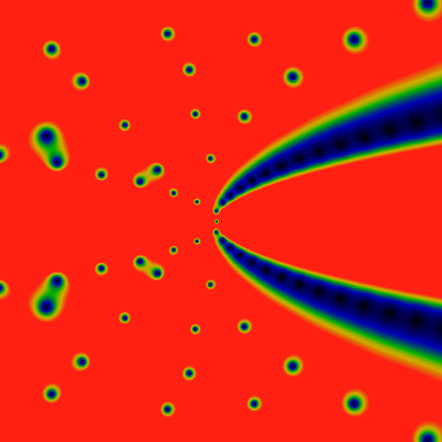
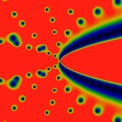
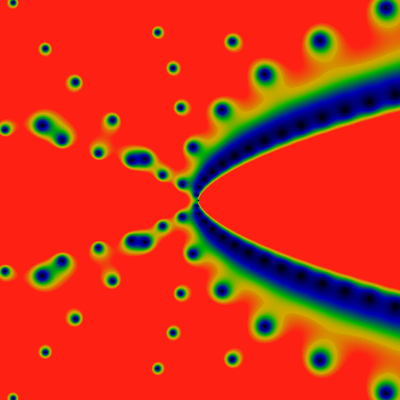
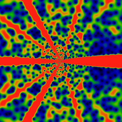
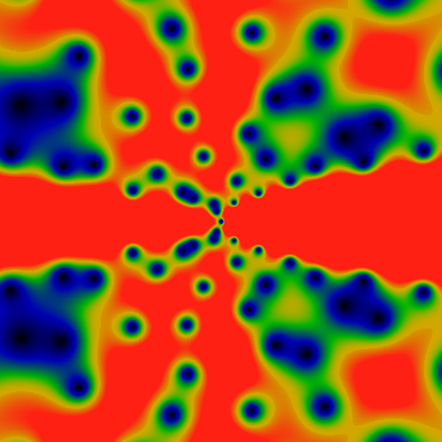
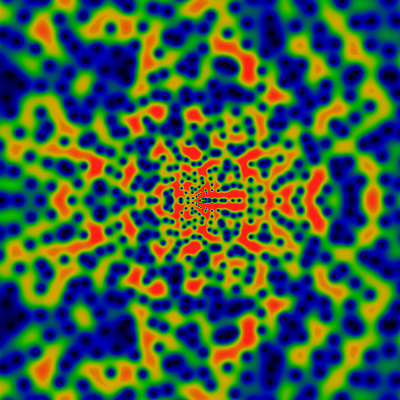
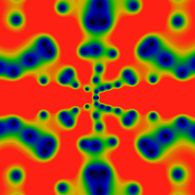
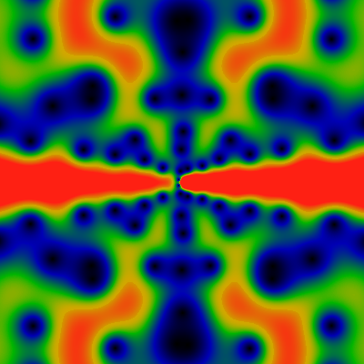
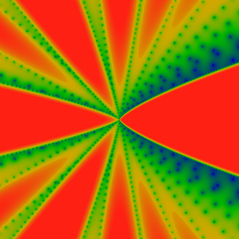
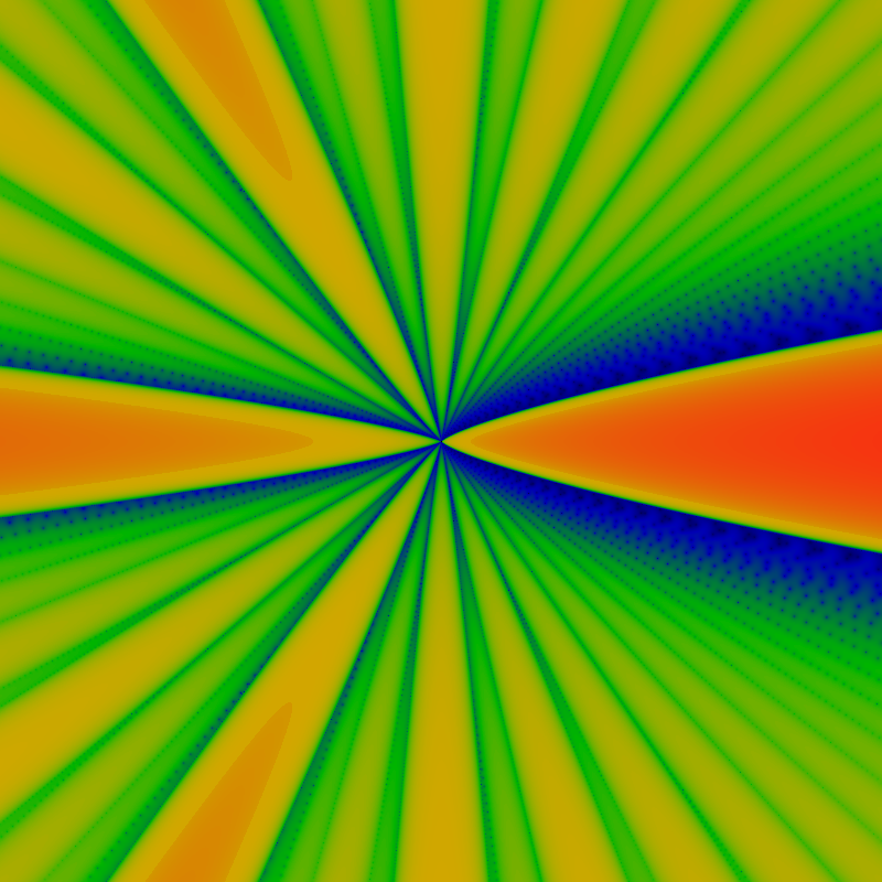
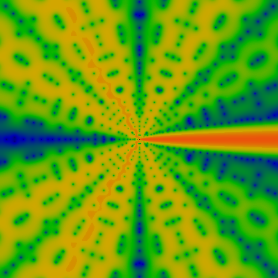
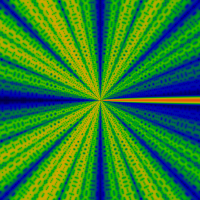
Lets start slow. Two images, both phase plots for Euler's totient function. On the left is the ordinary generating function; on the right is the exponential generating function.
The ordinary generating function is given by OG(f; z) = Σn=1∞ f(n) zn and the exponential generating function by EG(f; z) = Σn=1∞ f(n) zn / n! (Note these sums start at one, not zero). Here, f(n) is the arithmetic series of interest, the totient function for these images. Both images show the complex phase -- that is, the arctan(y/x), where G(f;z)=x+iy. The phase runs from -pi to +pi, and the coloration is such that black is -pi, green is zero, and red is +pi. The ordinary generating function shows only the unit disk: everything inside of |z|< 1. The exponential generating function shows a square, for a domain -30 ≤ x,y ≤ +30 for z=x+iy.
Of course, as the phase wraps around from +pi back to -pi, there is a red-black discontinuity. From basic complex analysis, everyone knows that the phase wraps around the zeros and the poles of a holomorphic function. Thus, each of the color-discontinuities in the pictures above end in either a zero or a pole. In fact, they are all zeros, and this can be readily discerned: the phase wraps around with the right-hand rule around zeros, going from red to black as one rotates in a right-handed fashion. Everything in sight is a zero.
Well, sort-of. The OG function is littered with poles at |z|=1. In fact, they even seem to be everywhere dense at |z|=1, preventing the analytic continuation past the unit disk. This corresponds to the surface being hyperbolic; the edge of the disk is hyperbolic infinity (if we were to, for example, endow the disk with the Poincare metric). No matter: every analytic function is harmonic (derivatives w.r.t the complex-conjugate coordinate z* vanish), and so we can endow the surface with geodesic rays and a metric. Anyway it appears that there are no poles for any |z|<1.
The primary topic of this page is the EGF, not the OGF, so we won't consider that any further (see the Numberetic Gallery for a very brief treatment). We are interested in the EGF, and where it's zero's lie.
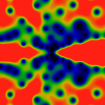
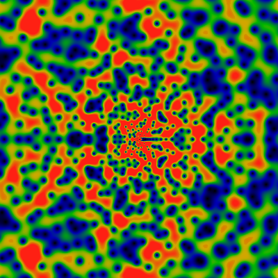
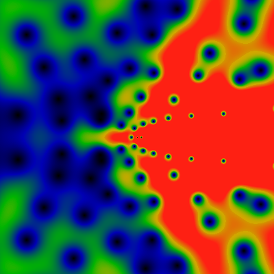
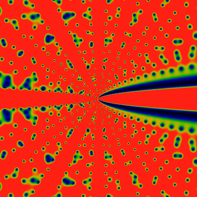
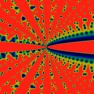
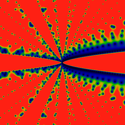
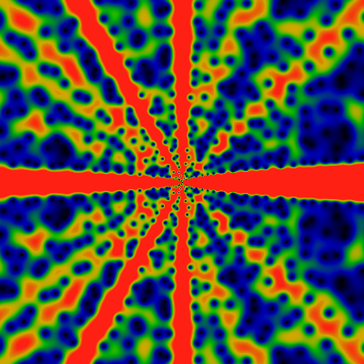
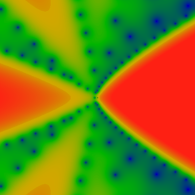
Can we get a better idea of the zeros? But of course we can! Good golly, Miss Molly! Have you ever seen such a thing before? I have not.
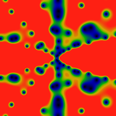
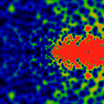
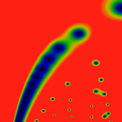
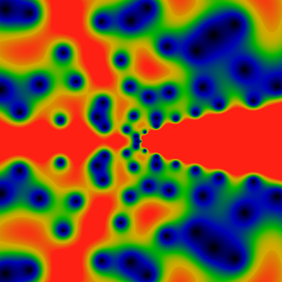
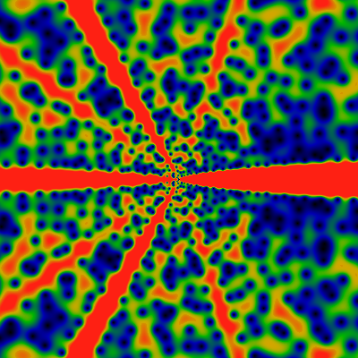
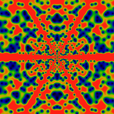
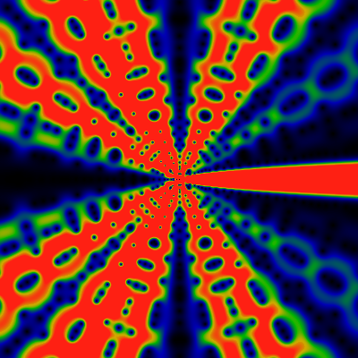
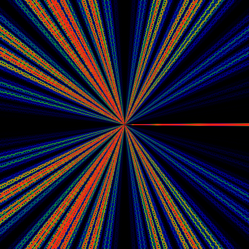
The above shows the magnitude of the exponential generating function of the totient function. The left image is over the domain -60 ≤ x,y ≤ +60 for z=x+iy, and the one on the right is for -500 ≤ x,y ≤ +500. The visualization is for the exponential generating function, normalized by its leading asymptotic behavior, which is exp|z|. That is, these pictures show |EG(f;z)| exp -|z| for f the totient function. The color scale is such that red represents values greater than 1.0, green represents values of about 0.5, and blue-black are values of 0.2 or less. The zeros are clearly visible as black dots. And, OMG, the zeros are spread out along rays. What is going on ???
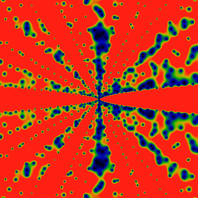
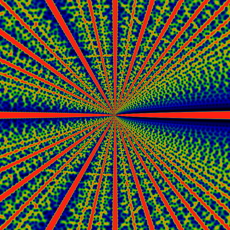
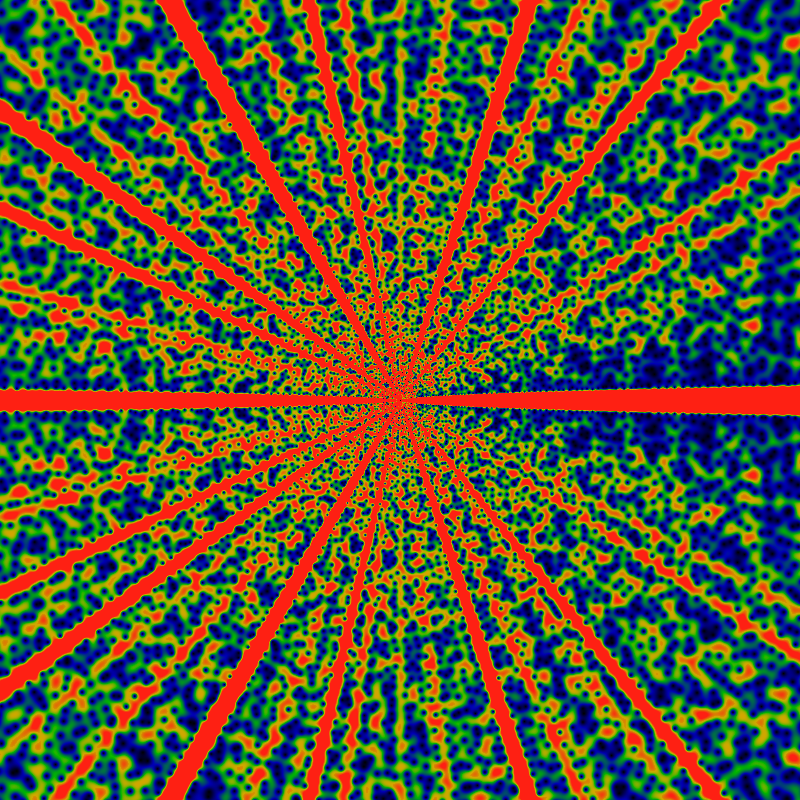
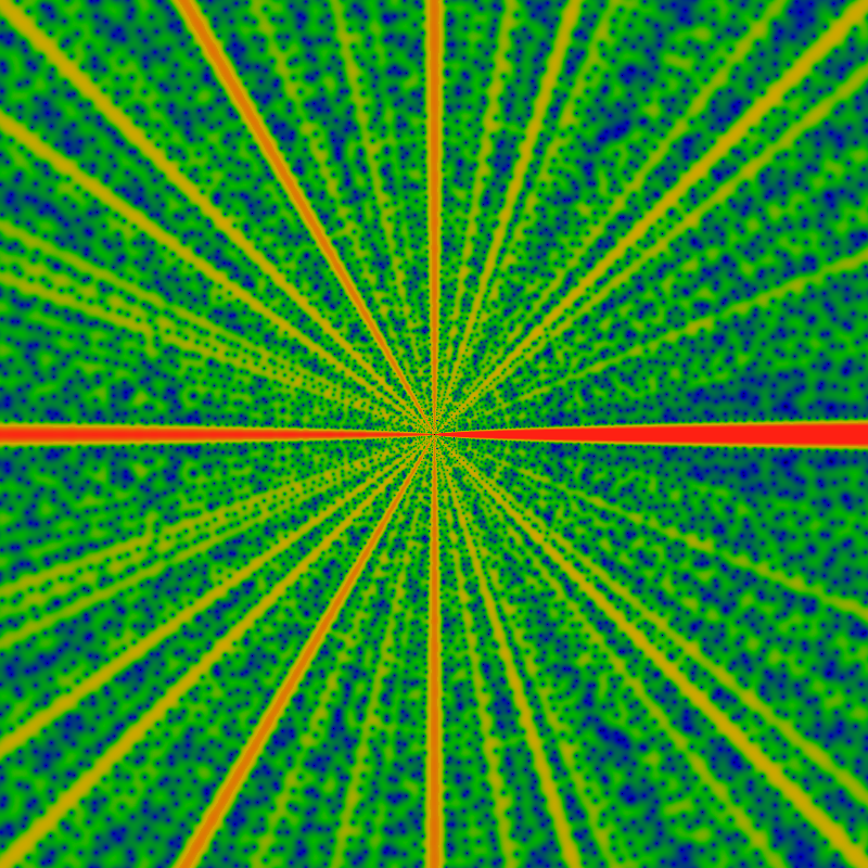
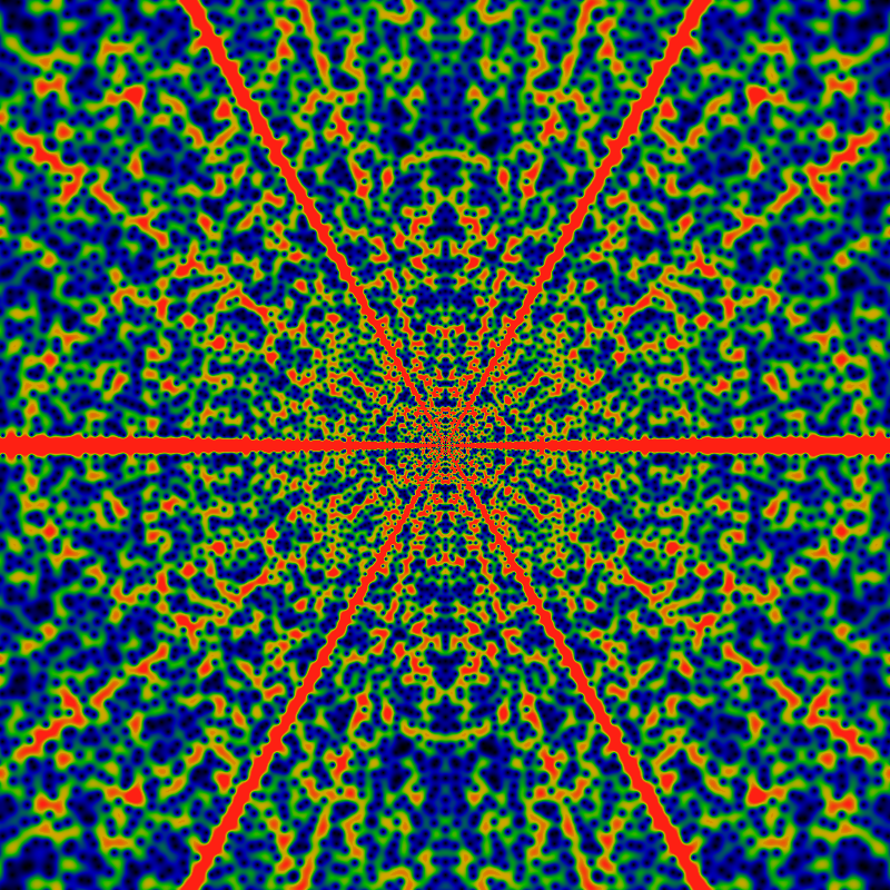
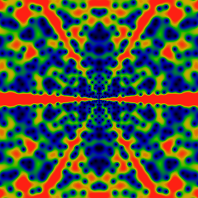
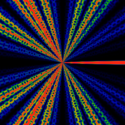
The below shows the same, for -6K ≤ x,y ≤ +6K. The color scale is chosen so that red corresponds to values of 1/15 or greater, green to values of about 1/30, and blue to values of about 1/60. Notable are lanes that are free of zeros, and anti-lanes that are filled with them. It is easiest to talk about angles as fractions of 2pi, so that angles run from 0 to 1 around the whole image, with the angle of 0 being the zero-free lane shooting off to the right from the center. Clearly, the lane 1/2 shooting straight-left from center is zero-free, but the anti-lanes 1/8, 1/4, 3/8 are clogged with zeros: I'd venture to guess that there is a clogged lane for each dyadic rational (each rational of the form m/2k).
You have to be a bit more observant to spot this, but clearly 1/3 and 2/3 are zero-free lanes, as are 1/5, 2/5, etc and 1/7, 2/7, 3/7, etc. If you look carefully, you can see that 1/9 and 2/9ths are zero-clogged: The 1/9 clog is just below the 1/8 clog which runs exactly to the diagonal, and the 2/9 clog is the next big one, just to the right of the 1/4 clog. You can verify this by fixing the location of the 1/3 lane, and observing that 1/9 and 2/9 trisect that angle. And so we are lead to a natural hypothesis: all lanes at an angle m/p for prime p are free of zeros, while those at angles m/pk for k>1 are clogged with zeros.
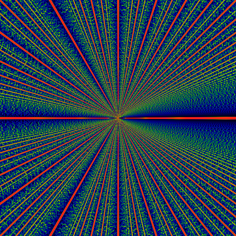
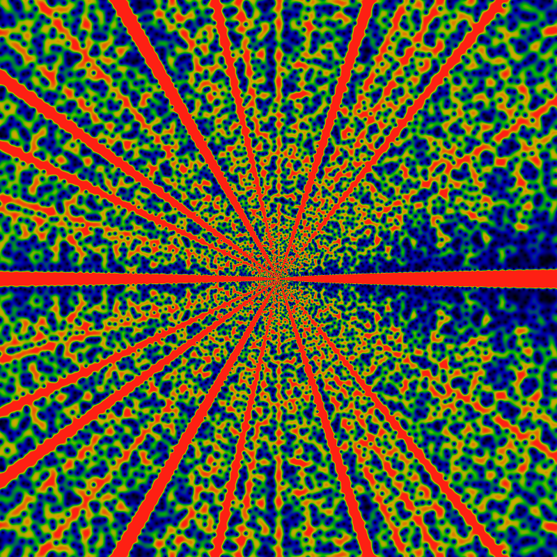
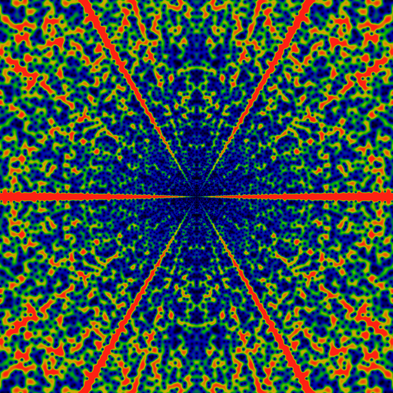
And again, for the domain -60K ≤ x,y ≤ +60K for z=x+iy. Visible in this image, while a lot less apparent in the previous images, is a rather regular, periodic stippling, especially in the anti-lanes that approach the angles of 0 and 1/2. If you look closely, you can spot some Moire patterning, which helps affirm the regularity of the stippling. The color scale is choose so that red corresponds to values of 1/8 or greater, green to values about 1/16, after dividing by the log-radius to help keep the color distributions well-balanced. That is, EGF(totient;z) appears to have an asymptotic behavior of EGF(totient;z)= O(exp |z| log |z|). In the earlier images, the divergence as exp |z| is removed, as it is quite overwhelming otherwise, but the much smaller logarithmic divergence was not corrected for, as it was not apparent. Here, the value of |z| gets so large, that the log is hard to miss. Its removal doesn't really make that much of a difference in these images: it simply makes the center redder or bluer, as compared to the edges.
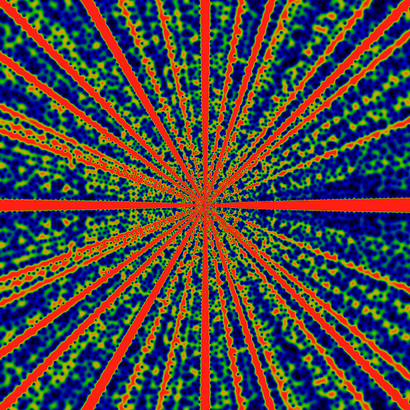
And so we embark on a general survey: Below is the Carmichael function, the exponent of the ring of units. It is similar to Euler's totient, so we expect some general similarity in the generating function, as well. So here: The two images show the domains -60 ≤ x,y ≤ +60 and -500 ≤ x,y ≤ +500. Red corresponds to 0.2 or greater. Well, there's one difference: the lanes of zeros are gone.
And here, again -- for -6K ≤ x,y ≤ +6K. Several differences, as compared to the totient function, can be observed. First, there are zero-free lanes at 1/4... but NOT at 1/8!. Huh. There do seem the be lanes at 1/5 and 1/6 and 1/7. Nothing in particular at 1/9 though. How is does this relate back to the arithmetic series?
And here, again -- for -60K ≤ x,y ≤ +60K. Again, a clear absence of the ray at 1/8. This seems to reverberate through the pattern. Compare to the divisor function, below, where no rays are ever suppressed.
Another quite famous function: Below is the Möbius function. The two images show the domains -60 ≤ x,y ≤ +60 and -500 ≤ x,y ≤ +500. Red corresponds to 6.0 or greater.
And here, again -- for -6K ≤ x,y ≤ +6K. There are vague, shadowy hints of large-scale structure, but nothing that pops out, not really. The distribution of zeros is really quite very uniform.
Zoom out -- for -60K ≤ x,y ≤ +60K. Same color scale as above. The fall-off to blue indicates that there is some weak asymptotic falloff, much less than logarithmic: so for example, a falloff of log(log |z|) is indicated, as log log 60K = 2.4 which is enough to bring the blue color back into the orange territory.
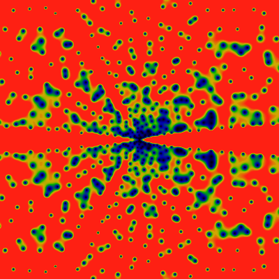
Below is the divisor function, it counts the number of divisors of n. The two images show the domains -60 ≤ x,y ≤ +60 and -500 ≤ x,y ≤ +500. Red corresponds to 4.0 or greater. Holy guacamole!
Below, again, for -6K ≤ x,y ≤ +6K. Red corresponds to 1.6 or greater. What are those non-radial bands that are trying to appear? The horizontal ones, the curvy ones. Wowee!
Below, again, for -60K ≤ x,y ≤ +60K. Red corresponds to 1.6 or greater. Notice the assorted fine tracery in the details.
Compared to the totient above, it appears as if there is a zero-free lane for each rational, or so it seems, at least, based on my quick eyeball impression. So, where are the zeros? The conjecture is -- only at the irrational angles. There is a vague hint that the width of the lanes can be ranked according to the position of those angles in the Farey tree: thus the widest is 0/1 then 1/2 then equally 1/3 and 2/3, then 1/4, 2/5, 3/5, 3/4, and so on. The lanes at 1/n get rapidly narrower, and the pile-up at the limit n->infty (the fat blue bands on the right) is characteristic of the Farey sequence, and things derived from it, such as the Minkowski Question Mark.
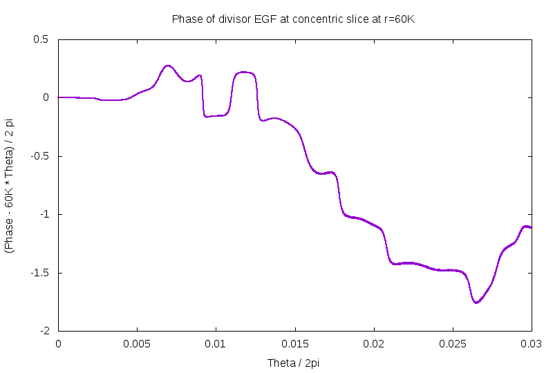
The last claim can be made clear: Here is a slice through the last image, at the fixed radius of r=60K. That is, it is a graph of the magnitude of generating function. Angles are labelled with the Farey fractions, and clearly, the heights fall into sequence.
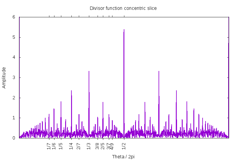
The Farey fractions form a fractal, the self-symmetry of which is generated by two functions: g(t)=t/(1+t) which maps the unit interval into the half-interval, and r(t)=1-t, which is a reflection about 1/2. The general element of the fractal self-similarity monoid is given by γ = gm rgn ... rgk where m,n,...,k are integers, and writing symbols next to each other is understood as function composition. This monoid is the "dyadic submonoid" of the modular group SL(2,Z), and has many other interesting representations, as well. I have numerous writings devoted to it, where more information can be found.
In this case, the self-similarity suggests that the generating function EGF(div, r exp(i2π t)) should be about the same as EGF(div, R(r,t) exp(i2π γ(t))) for any γ in the dyadic monoid, and some suitable R(r,t) that depends on gamma. However, this cannot hold in this naive way, because any mapping from z = r exp(i2π t) to Z(r,t) = R(r,t) exp(i2π γ(t)) cannot be be holomorphic unless gamma is a linear function of t, and gamma is certainly not linear. That is, Z(r,t)=Z(z,z*) will depend on z* in general. The apparent self-similarity is not, cannot be merely a holomorphic re-mapping of one pie-slice into another. Whatever it is, it is more subtle than this.
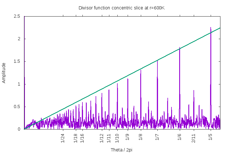
Are the peaks in linear proportion? Visually, the needles in the image above seem to have heights that are not quite in linear proportion. Is this an artifact of some sort? Below is a high-precision examination of the peak heights. Unlike the previous figure, the slice here is taken at r=600K, so much farther from the origin, making the peaks narrower and hopefully more asymptotic. The digital sampling is fine enough such that the peak at 1/5 is sampled by several dozen points, and so the graphed height really does accurately show the true height. The straight line is drawn with a slope of 1.7. As can be seen, the peaks at 1/6 and 1/5 exceed it, while all the others fail to reach up to the line.
But this figure may be deceiving. Each of the peaks represents a lane, and the lanes are slowly (logarithmically?) diverging as a function of the radius. The asymptotic form of this divergence is not known. Thus, it is not clear how much of this figure is muddled by the non-leading terms in the asymptotic expansion.
So, what is the dyadic tree? The image below illlustrates it. Its just an ordinary binary tree: here, its illustrated with fractions that have powers of two in the denominator; there is also an equivalent Stern-Brocot tree tree with the Farey fractions appearing on it. The dotted golden lines extend from nodes on the tree to the cusps. Notice that each blue edge, together with two golden lines, forms a triangle. This triangle is commonly refered to as the fundamental domain. The cusp is the point of the triangle that is located at "infinity". Notice that an infinite number of triangles share a cusp point, and that the golden lines necessarily accumulate or bunch up to form a lane down the gaps in the binary tree.

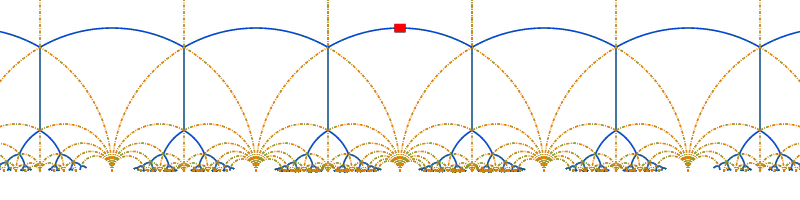
There is a very traditional mapping of this tree into the upper half-plane, shown in the image below. The same color scheme is used, the vertex labels are omitted. The red rectangle is understood to be the root of the tree, i.e. corresponding to the label "1/2" in the previous image. That is, the tree is unfolded into left and right halves. The point here is that this is (homotopically) equivalent to the previous diagram: its the same tree, the same cusps, just a diferrent layout: the upper half-plane is customarily given a hyperbolic (Poincaré) metric.
What, exactly, is the point here? The claim, the hypothesis, here is that the zero-free lanes in the EGF of the divisor function correspond exactly to the cusps of the binary tree. There is even a stronger claim buried in here: that the zeros of the EGF of are in one-to-one correspondance with the funamental domains of the binary tree. To be even more precise, there is exactly one zero at each vertex of the binary tree. This even provides a "natural" explanation for why the zero-free lanes are of finite width: they need to be wide enough to accomadate an ever-growing number of cusp lines.
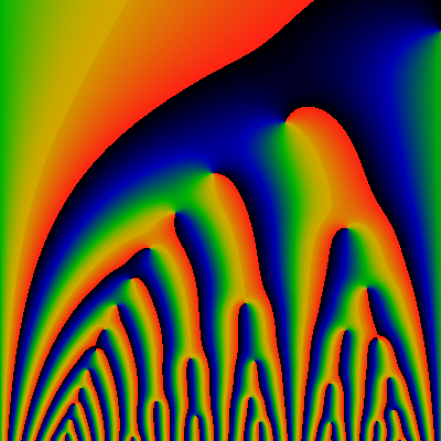
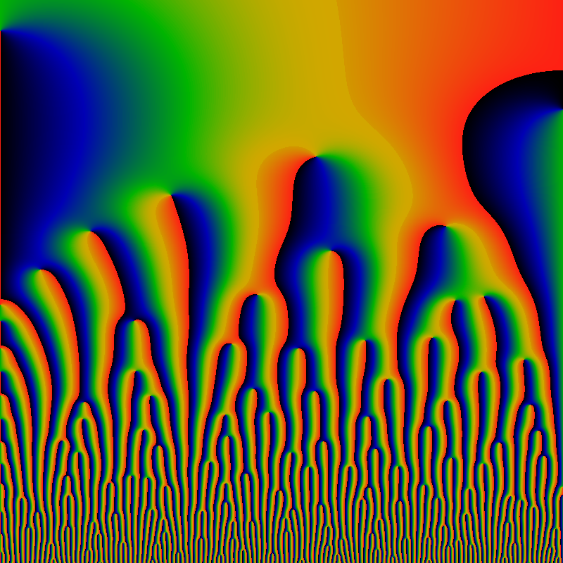
This is illustrated most clearly below. The next pair of images show the divisor function, again -- this time, unwound into a rectangle, so that the coordinates are given by z=r exp(i theta) with theta running from zero to pi, left to right, and r running from 1 at the top, to 64 at the bottom, on a logarithmic scale. The left image should be clearly recoginizable from before. The right image shows the same area, but as a phase plot That is, it shows the phase phi=arctan(Im EGF/ Re EGF) for EGF(z; div). The colors map over the range zero to two-pi of the phase of the EGF. Black is zero or a bit more, green is near pi, and red is just less than 2pi, and a black-red transition is where the phase wraps. Thus, a zero is a point where the all the colors circulate around, wrapping around in a right hand manner (a pole would have the colors winding around in a left-handed fashion; but there are no poles here, only zeros.) Thus, each red-black transition terminates at a zero.
This phase diagram is glorious ... and deceptively misleading. Looking at the first few, most prominent zeros, there seems to be an "obvious" pattern: each red-black transition corresponds to one of dotted-golden cusp lines from the drawing above. A second dotted-golden cusp line runs down the middle of each green stripe. These form two of the edges of a fundamental domain; the third side is a line of constant phase, connecting zeros to what should be an obvious left and right. But is it really obvious, or even correct?
No, its not. Following the line of zeros arcing down the left side, one eventually realizes that there is something funny going on: there's a skip pattern. Some of the zero-phase lines go off to the left, other head right. The pattern seems regular, but doesn't alternate, nor is it necessarily every third one... The lines of phase equal to pi (green) -- where are they heading? There's some regular pattern, alright, but not as regular as the binary-tree-with-cusps idea suggests. There's something snarkier going on here.
One can try to hold out some hope: Klein's j-invariant has triple-zeros at the binary-tree vertexes. Here, we have simple zeros, so perhaps the phase lines at 0, 2pi/3 and 4pi/3 sketch out the desired tree?
Here's a very short table of the first five zeros. The table is in the format z=r exp(i π φ) = x + i y, with accuraccy to roughly the last printed digit. Plouffe's inverter doesn't seem to know any of these numbers. They're presumably all some unknown transcendentals.
| r | φ | x | y |
|---|---|---|---|
| 1.32445069102560611856977 | 1 | 1.32445069102560611856977 | 0 |
| 3.13928330237309484149222 | 0.64577556427965429878310 | -1.3879584941586381640249 | 2.81578956441198027350171 |
| 5.09769633868922933247499 | 0.48168974269433751784449 | 0.29307498156146120080527 | 5.08926468329839601692358 |
| 7.43590742268481661295516 | 0.39632841386773226736599 | 2.37923961785136162268330 | 7.04499382821487350822554 |
| 8.55373992551888671794606 | 0.78670383666114725404025 | -6.7041304003889043557580 | 5.31235374273938563634214 |
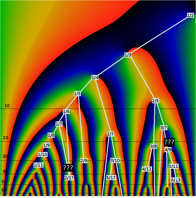
Below is an attempt to force a mapping of the Stern-Brocot tree onto the image. It starts out OK, and then things get confused. The node labelled 1/6th breaks the pattern... I've placed a question mark at the point of confusion. So, for example, there seems like there should be a curve of constant phase, connecting the zero at 1/3 to that at 2/5. Likewise for 1/4 and 2/7. Maybe (or maybe not) for 1/5 and 2/9. But .. it also looks like there might be a curve of constant phase joining up 1/6 to 2/9 .. and none at all joining 1/6 to 2/1? The naive tree mapping is not working out.
Below is the table of zeros matched to the labels. The column "farey" is the Stern-Brocot label; The clumn marked "dyadic" would be the corresponding dyadic-tree label (where the denominators are always a power of two). The "min" and "max" columns provide the left and right parent of a fraction; the Farey fraction is the Farey-sum of the min and max values.
The hypothesis here is that the angle φ obeys 2 min ≤ φ ≤ 2max and that φ should be "near" twice the Farey number. That is, in some sense, we expect that the numerical value of φ should be twice the numerical value of the Farey number. Of course, it isn't, so the column d shows the difference between the expected and the actual value, rescaled by the distance to the min/max bound. So, for example, in the third row, d = 3 * (0.64577 /2 - 1/3) = -0.03133 so the actual zero is 3 percent to the left of its expected location.
Sadly, this hypothesis does not hold. First, there is skip behavior, already noted as occuring at 1/6. The same skip pattern suggests that the zero marked 4/9 is in fact mis-labelled. Indeed the zero is not where one might guess: the zero for 4/9 is too far over to the left -- it is left of the lower bound of 3/7. Whoops!
| Dyadic | Farey | Min | Max | r | φ | d |
|---|---|---|---|---|---|---|
| 0/1 | 0/1 | - | - | 0 | - | - |
| 1/2 | 1/2 | 0/1 | 1/1 | 1.32445069102560611856977 | 1 | 0 |
| 1/4 | 1/3 | 0/1 | 1/2 | 3.13928330237309484149222 | 0.64577556427965429878310 | -0.03133665358051855182534 |
| 1/8 | 1/4 | 0/1 | 1/3 | 5.09769633868922933247499 | 0.48168974269433751784449 | -0.03662051461132496431102 |
| 3/8 | 2/5 | 1/3 | 1/2 | 8.55373992551888671794606 | 0.78670383666114725404025 | -0.09972122504139559469808 |
| 1/16 | 1/5 | 0/1 | 1/4 | 7.43590742268481661295516 | 0.39632841386773226736599 | -0.00917896533066933158502 |
| 3/16 | 2/7 | 1/4 | 1/3 | 17.3953078163703147248202 | 0.55588972866838613293425 | -0.21754379864259413892038 |
| 5/16 | 3/8 | 1/3 | 2/5 | 22.3706980126923113903896 | 0.78276436269888310039513 | +0.65528725397766200790279 |
| 7/16 | 3/7 | 2/5 | 1/2 | 15.0696161657378566235666 | 0.83030753160631370834127 | -0.46961819688951010402768 |
| 1/32 | 1/6 | 0/1 | 1/5 | 10.3697073593993873720516 | 0.33911521638363347825296 | +0.08672824575450217379451 |
| 3/32 | 2/9 | 1/4 | 1/5 | 29.1983628540125538782212 | 0.43237645839168297310565 | -0.27152968618713310512268 |
| 15/32 | 4/9 | 3/7 | 1/2 | 24.6490878240833776657973 | 0.85616009823198724723879 | -1.03095690569240171197796 |
| 1/64 | 1/7 | 0/1 | 1/6 | 13.8146212377999426722697 | 0.29636827418504324576301 | +0.22373375788590816102324 |
| 1/128 | 1/8 | 0/1 | 1/7 | 17.7592747006298291624242 | 0.26340458841672307306728 | +0.37532847566824604588406 |
Despite this failure, there are still two interesting ways to correlate zeros and angles. So first: consider a circle, centered on the origin. Assume no zeros lie on the circle. The EGF will have some phase on every point on the circle; one can now trace curves (geodesics) of constant phase, inward towards the origin. Each such curve must land on some zero -- almost all such curves will land on a circle, although a few will encounter saddlepoints and split. Thus, effectively each point on the circle can be associated (almost always) uniquely with some zero inside that circle. So, what does the graph of zeros look like?
Consider now tracing curves of constant phase in the opposite direction: starting at each zero, trace all possible phase lines, and see where they go, with increasing radius. In general, this set will not be a connected set: it will terminate on a set of intervals on the circle. What are these intervals? How many of them are there? (It seems that they will be self-similar fractals, scopficially, Cantor sets, in general) What is the min and max angular extent of this set? Can the min and max extent be used to label the corresponding zero with a unique Farey fraction?
These questions can be explored numerically, but take more work.
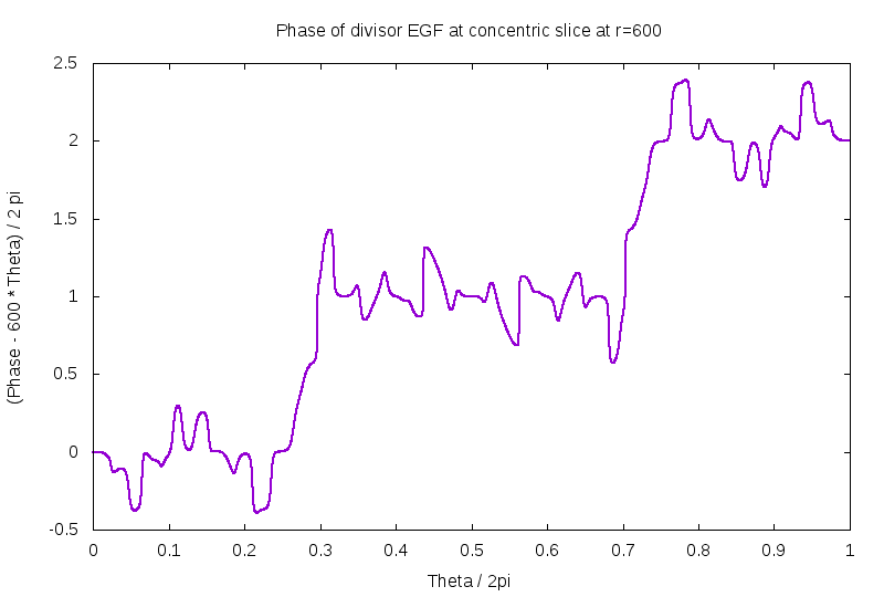
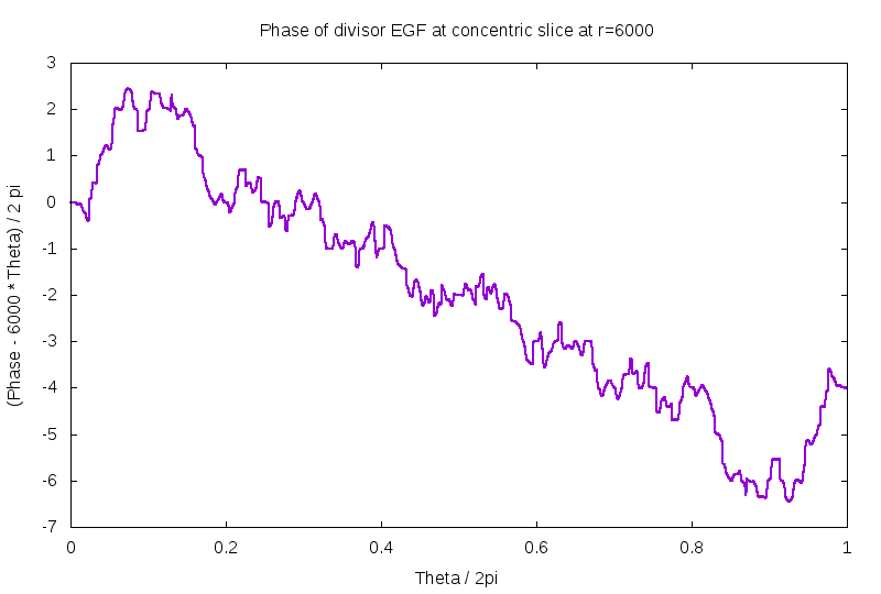
So: what is the phase actually like? Well, for starters, for a circle of radius r, there are approximately r zeros inside of it. This is established elsewhere here, or on the GPF page. This approximation is fairly good, being off by less than log(r) and maybe just log(log(r)) or so. Therefore, as one travels around the perimeter of the circle, one expects that the phase change roughly as the radius times the angle along the circle. Subtracting this leading term, one gets the figures bewlo, first for r=600, the second for r=6K. Apparently, there are 602 zeros inside a circle of radius 600, but only 5996 zeros inside a circle of radius 6K. Other than that, these two figures indicate that the phase behaves in a rather other-wordly fashion. The mis-shapen bumps and lumps are ... unexpected and unusual. I guess some of this is just due to the circle flying close to some zeros?
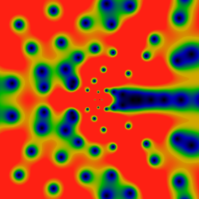
If you're like me, the next question is: what's up with the EGF for the Mobius function? It has no rays. What is it doing? In all glory, the answer is below. zero to pi, left to right, and r runs from 1 to 256 on a log scale, top to bottom. There is, for lack of a better term, "bifurcations" all the way down, but these seem to be arranged to be evenly distibuted.
By the way: I have no direct evidence here, but some quick experiments indicate that almost all random (randomly generated) arithmetic series (with sutiably bounded growth rates, etc) seem to behave much like this. This is important: as much of what seems to be special on this and the GPF page are in fact common properties enjoyed by most sequences.
Now that we are on this topic, how do things compare for the totient function? The situation is similar, but diffferent. First, notice the completely different scale of the divergences of the lanes: the slice taken here is at r=60K.
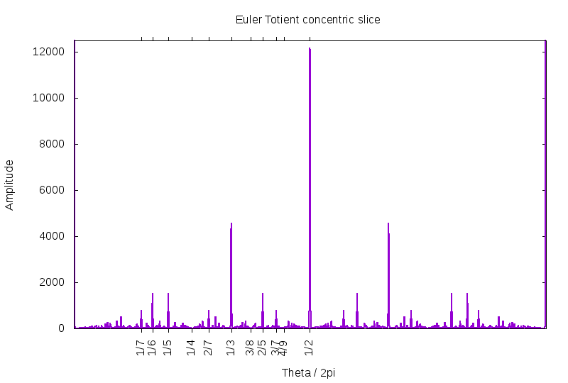
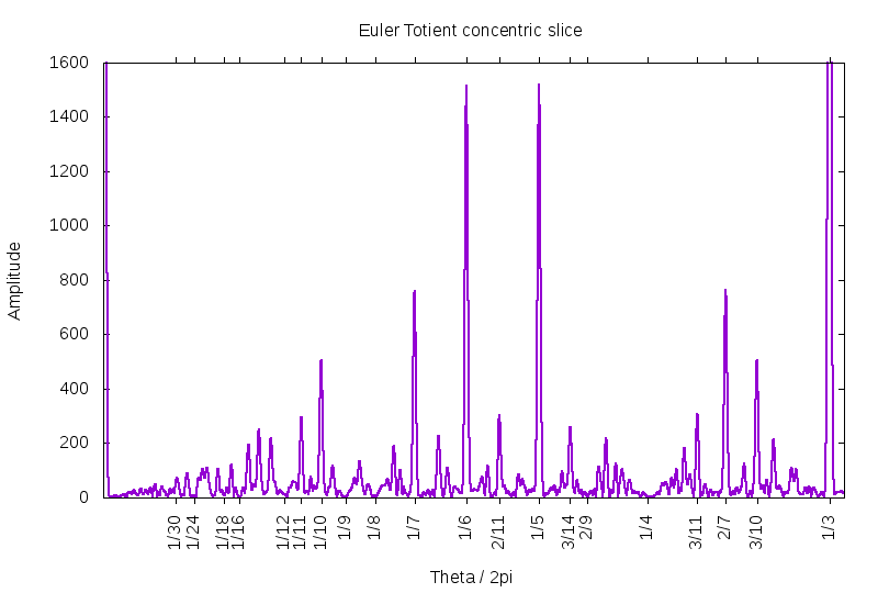
Next, notice that peaks are absent, whenever the denominator of a Farey fraction has more than one power of a prime in it. That is, there is a complete absence of peaks at 1/4, 1/9, etc. as well as 1/8, 1/12, etc. This is more clearly demonstrated below, which just zooms in on the lower reaches. Does this mean that there are one or more zeros located at these angles? Or do zeros simply gather close to these angles? Unknwon. The equal heights of the lanes at 1/5 and 1/6 are a bit confounding, especially compared to the peak at 1/7. The peak at 1/6 gets a boost, is that due to having two prime factors? This suggests that the peak at 1/30 might get a boost as compared to its neighbor at 1/26, but that is not evident, in this figure.
What about powers of the divisor function? See below, for for -60 ≤ x,y ≤ +60, for sigma-one on the left, sigma-two on the right.
Although they look very similar, they are not the same. The zeros are in slightly different positions. This is particularly evident at close-range; father away, the differences are relatively smaller, as shown below, for the domain -500 ≤ x,y ≤ +500.
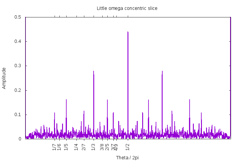
Below are the two Prime factor counting functions. Little omega (OEIS A001221) counts the number of distinct prime factors, while big omega (OEIS A001222) counts the total number of prime factors. of n. The images show the domains -60 ≤ x,y ≤ +60 and -500 ≤ x,y ≤ +500, as always. First, the "little omega": red corresponds to 4.0 or greater.

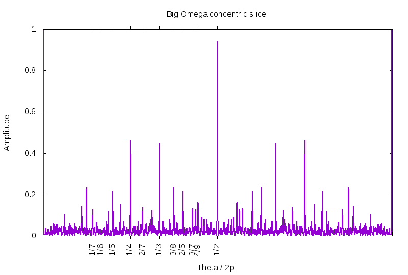
Next, the "big omega". Red corresponds to 4.0 or greater.
Next, the unitary divisor function, which is the same as 2 to the power little-omega. You might think that the unitary divisor would resemble the divisor function itself, but no. (Recall, the unitary divisor is the divisor, but with gcd of non-unit factors excluded). Red corresponds to 2.0 or greater.
Little omega, again, for -6K ≤ x,y ≤ +6K, and red being values of 16.0 or greater. A mixture of lanes and anti-lanes at different rational angles. If you blur your eyes a bit, you can make out vague hints of a concentric ring structure. It seems to be there, but there is no remaining evidence after a zoom-out.
The unitary divisor, red being 3 or greater. Its remarkable how similar the unitary divisor is to little-omega, although, if you look carefully, you can see that it has lanes which little omega does not.
Big omega, again, for -6K ≤ x,y ≤ +6K. Here, as well, there is a hint of concentric ring structures.
Big omega, as above, but with a softer color palette. This shows the 4th root of the magnitude, so that large values are lowered toowards 1.0, while small values are raised twoards 1.0. The color interpretation is same as always: green corresponds to values around 0.5, and red to those above 1.0.
The softening makes the location of the zeros far more distinct. It also gives a hint of the relative strength of the divergences of the various rays: Clearly, 0 and 1/2 are strong, 1/3 competes with 1/4th for divergence strength.
Graphs of the magnitude of the EGF of the little and big omega functions, at the radius of r=60K.
Below is the Liouville lambda function, given by (-1) to the power of the Big omega: thus, it is always +1 or -1. The two images show the domains -60 ≤ x,y ≤ +60 and -500 ≤ x,y ≤ +500. Red corresponds to 4.0 or greater. Note the overall general resemblance to the Moebius mu.
Below is the Von Mangoldt lambda function, the log of p if n=pk for some prime p and integer k The two images show the domains -60 ≤ x,y ≤ +60 and -500 ≤ x,y ≤ +500. Red corresponds to 4.0 or greater.
Again, for -6K ≤ x,y ≤ +6K. Quite unlike any of the other images above, this one appears to have a left-right symmetry. Do not be fooled: this is not so; there is a very slight asymmetry: It can only be seen in the above-left image for the -60 ≤ x,y ≤ +60 domain. There, you can see that the function is trying hard to be left-right symmetric, but failing: close, but no cigar. Any evidence of that asymmetry is gone, once one zooms out a bit more.
Below is the exp of the Von Mangoldt lambda function, that is, the function that is p if n=pk for some prime p and integer k, else it is 1. The two images show the domains -60 ≤ x,y ≤ +60 and -500 ≤ x,y ≤ +500. Red corresponds to 1/4 or greater. Note the overall general resemblance to the regular Von Mangoldt lambda. In addition to diverging exponentially (like all the other functions on this page), this seems to also have a much softer log2|z| divergence, which is divided out go give a better color balance between the areas with large and small |z|.
Again, for the domain -6K ≤ x,y ≤ +6K. This one is conspicuously missing rays at 1/4 and other powers of 2. There is nothing obvious about the Von Mangoldt lambda that would hint at why this would be the case.
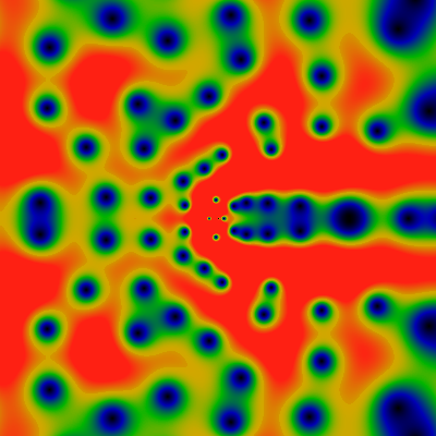
Below is the partition function or "integer partition", the various ways in which an integer can be decomposed into parts.
The first, image, as usual, runs over -60 ≤ x,y ≤ +60. Coloring this was tough, because large portions of the plane are close to zero, while other parts are strongly divergent. A naive coloring was alternating black and red. To bring out the colors, the 6th root of the magnitude was taken -- thus, small values are sharply drawn up towards 1.0, and large values are sharply pushed down towards 1.0. After this, green corresponds to values of about 0.4, and red to values of about 0.8 or greater.
Again, for -500 ≤ x,y ≤ +500. Obviously, there are some extremely wide rays that appear to be centered on the simple rational fractions. How wide are they, and where are the zeros?
Here's a very short table of the first four zeros. The table is in the format z=r exp(i π φ) = x + i y, with accuraccy to roughly the last printed digit. Plouffe's inverter doesn't seem to know any of these numbers. They're presumably all some unknown transcendentals.
| r | φ | x | y |
|---|---|---|---|
| 4.326780701337451813049818 | 0.513591485509299027015766 | -0.18469269040171525788985 | 4.322837013765194865400579 |
| 6.958191756899281112787412 | 0.460442316538141512940103 | 0.862499123470730812758174 | 6.904529512413812938143440 |
| 8.326620629311171748261946 | 0.768253588902337962587366 | -6.21558501059661474242568 | 5.540678124608670537285123 |
| 9.783425570675309270218631 | 0.411350237714961115696809 | 2.689611824379544750067657 | 9.406455449907857709201997 |
Again, for -6K ≤ x,y ≤ +6K.
Below is the Thue-Morse sequence, the period-doubling sequence that generates the Cantor-set sequence. The two images show the domains -500 ≤ x,y ≤ +500 and -6000 ≤ x,y ≤ +6000. Notice this is much wider than the previous images, above. The narrow view is boring. Red corresponds to 12.0 or greater.
Using the same colormap-rescaling trick as described earlier, here are the same two pictures as above, with softened contrast. This helps make clear that there were more zeros hiding in the dark bands.
And here, again -- for -60K ≤ x,y ≤ +60K. I just love the digital precision in these images!
The greatest prime factor function enjoys a much greater, in-depth analysis, and gets it's own page. See the greatest prime factor gallery. Below is a movie trailer for that show:
Initial version: October 2016

Greatest Prime Factor
by Linas Vepstas is licensed under a Creative Commons
Attribution-ShareAlike 4.0 International License.